- 8.32 Neil Shah
December 4, 2019
Meetup Presentations
Bayesian Analysis

Kruschke’s videos are an excelent introduction to Bayesian Analysis https://www.youtube.com/watch?v=YyohWpjl6KU!
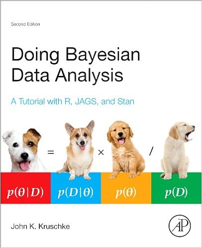
Doing Bayesian Data Analysis, Second Edition: A Tutorial with R, JAGS, and Stan
The Theory That Would Not Die: How Bayes’ Rule Cracked the Enigma Code, Hunted Down Russian Submarines, and Emerged Triumphant from Two Centuries of Controversy by Sharon Bertsch McGrayne
Bayes Theorem
\[ P\left( A|B \right) =\frac { P\left( B|A \right) P\left( A \right) }{ P\left( B|A \right) P\left( A \right) +P\left( B|{ A }^{ ` } \right) P\left( { A }^{ ` } \right) } \]
Consider the following data from a cancer test:
- 1% of women have breast cancer (and therefore 99% do not).
- 80% of mammograms detect breast cancer when it is there (and therefore 20% miss it).
- 9.6% of mammograms detect breast cancer when it’s not there (and therefore 90.4% correctly return a negative result).
| Cancer (1%) | No Cancer (99%) | |
|---|---|---|
| Test postive | 80% | 9.6% |
| Test negative | 20% | 90.4% |
How accurate is the test?
Now suppose you get a positive test result. What are the chances you have cancer? 80%? 99%? 1%?
- Ok, we got a positive result. It means we’re somewhere in the top row of our table. Let’s not assume anything - it could be a true positive or a false positive.
- The chances of a true positive = chance you have cancer * chance test caught it = 1% * 80% = .008
- The chances of a false positive = chance you don’t have cancer * chance test caught it anyway = 99% * 9.6% = 0.09504
| Cancer (1%) | No Cancer (99%) | ||
|---|---|---|---|
| Test postive | True +: 1% * 80% | False +: 99% * 9.6% | 10.304% |
| Test negative | False -: 1% * 20% | True -: 99% * 90.4% | 89.696% |
How accurate is the test?
\[ Probability = \frac{desired\quad event}{all\quad possibilities} \]
The chance of getting a real, positive result is .008. The chance of getting any type of positive result is the chance of a true positive plus the chance of a false positive (.008 + 0.09504 = .10304).
\[P(C | P) = \frac{P(P|C) P(C)}{P(P)} = \frac{.8 * .01}{.008 + 0.095} \approx .078\]
So, our chance of cancer is .008/.10304 = 0.0776, or about 7.8%.
Bayes Formula
It all comes down to the chance of a true positive result divided by the chance of any positive result. We can simplify the equation to:
\[ P\left( A|B \right) =\frac { P\left( B|A \right) P\left( A \right) }{ P\left( B \right) } \]
How many fish are in the lake?
- Catch them all, count them. Not practical (or even possible)!
- We can sample some fish.
Our strategy:
- Catch some fish.
- Mark them.
- Return the fish to the pond. Let them get mixed up (i.e. wait a while).
- Catch some more fish.
- Count how many are marked.
For example, we initially caught 20 fish, marked them, returned them to the pond. We then caught another 20 fish and 5 of them were marked (i.e they were caught the first time).
Adopted from Rasmath Bääth useR! 2015 workshop: http://www.sumsar.net/files/academia/user_2015_tutorial_bayesian_data_analysis_short_version.pdf
Strategy for fitting a model
Step 1: Define Prior Distribution. Draw a lot of random samples from the “prior” probability distribution on the parameters.
n_draw <- 100000
n_fish <- sample(20:250, n_draw, replace = TRUE)
head(n_fish, n=10)
## [1] 153 67 41 82 90 103 54 48 86 167
hist(n_fish, main="Prior Distribution")
Strategy for fitting a model
Step 2: Plug in each draw into the generative model which generates “fake” data.
pick_fish <- function(n_fish) { # The generative model
    fish <- rep(0:1, c(n_fish - 20, 20))
    sum(sample(fish, 20))
}
n_marked <- rep(NA, n_draw)
for(i in 1:n_draw) {
    n_marked[i] <- pick_fish(n_fish[i])
}
head(n_marked, n=10)
## [1] 3 8 13 5 4 7 8 8 5 2
Strategy for fitting a model
Step 3: Keep only those parameter values that generated the data that was actually observed (in this case, 5).
post_fish <- n_fish[n_marked == 5]
hist(post_fish, main='Posterior Distribution')
abline(v=median(post_fish), col='red')
abline(v=quantile(post_fish, probs=c(.25, .75)), col='green')
What if we have better prior information?
An “expert” believes there are around 200 fish in the pond. Insteand of a uniform distribution, we can use a binomial distribution to define our “prior” distribution.
n_fish <- rnbinom(n_draw, mu = 200 - 20, size = 4) + 20
hist(n_fish, main='Prior Distribution')
What if we have better prior information?
n_marked <- rep(NA, n_draw)
for(i in 1:n_draw) {
    n_marked[i] <- pick_fish(n_fish[i])
}
post_fish <- n_fish[n_marked == 5]
hist(post_fish, main='Posterior Distribution')
abline(v=median(post_fish), col='red')
abline(v=quantile(post_fish, probs=c(.25, .75)), col='green')
Bayes Billiards Balls
Consider a pool table of length one. An 8-ball is thrown such that the likelihood of its stopping point is uniform across the entire table (i.e. the table is perfectly level). The location of the 8-ball is recorded, but not known to the observer. Subsequent balls are thrown one at a time and all that is reported is whether the ball stopped to the left or right of the 8-ball. Given only this information, what is the position of the 8-ball? How does the estimate change as more balls are thrown and recorded?
shiny_demo('BayesBilliards', package='DATA606')
See also: http://www.bryer.org/post/2016-02-21-bayes_billiards_shiny/